


An Example of Shor's Factoring Algorithm

You may have heard of Shor’s algorithm, a quantum algorithm that can find factors of a number on a quantum computer. It is widely believed that a quantum version of factoring algorithm can allow for a faster cracking of encryption providing a speedup over classical factoring algorithms. When it comes to securing encryption keys, we need to find the prime factors of a number. Prime numbers are those that are only divisible by themselves and 1, examples being 11, 5, 31, and so on.
In this article, I aim to provide a practical guide to Shor’s factoring algorithm without delving into an extensive theory that can be easily found on the Internet. This guide is particularly useful for those who are already familiar with the theory of Shor’s algorithm and are seeking some practice. On the other hand, for those who prefer a hands-on approach, you might find it helpful to first blindly follow my example and then check my work and deepen your knowledge through reading a more thorough theory of Shor’s factoring algorithm.
Prerequisites. This is an intermediate-level tutorial that assumes familiarity with quantum computing principles such as superposition, measurements, quantum gates, and QFT. It is also suitable for people with extensive math backgrounds but with little or no prior knowledge of quantum computing.
Problem.
Given a number K=39, find out its prime factors using Shor’s factoring algorithm.
Solution.
Step 0. To begin with, we need to set up all the required variables and choose some initial values. We have an integer K=39, and our objective is to find its prime factors — factors that are neither 1 nor 39. While it’s easy to determine such factors for K=39 as 3 and 13, finding prime factors of larger numbers can be a difficult task. Let’s name these factors c and d, such that K=c*d. Our goal is in finding these numbers c and d using a quantum computer. For educational purpose, we can use 3 and 13 as the reference to check our work later.
Now, since we don’t know the values of c and d, we start with a guess a=5 . . . This could sound non-scientific but Shor’s algorithm will eventually turn out our guess into a correct factor. The initial guess of a factor could be any number less than the number we want to factor out, a < K, and which shares no common divisors with K. We could even guess one of the factors of K, or another factor that shares a factor with K but the larger K is the less likely we are to guess correctly.
If we take our guess and raise it to some power N, we can get the multiples of K plus 1:

We will need a slightly modified version of this expression: we subtract 1 from both sides and then factor out the expression using the difference of squares formula: x² — y² = (x — y)(x + y):

By doing so we have introduced some restrictions on N. Eventually,

would be the factors of K. The K is an integer and we are interested in finding integer factors of K, thus, we can not allow N to be an odd number. So N must be even (N has to have 2 as its factor). If N is odd, then raising a to odd N/2 would make no sense in our calculations.
N in this case can be thought of as an order of numbers a and K (a^N mod K =1) while 1/N represent the frequency in the Quantum Fourier transformation that we will deal in Step 5.
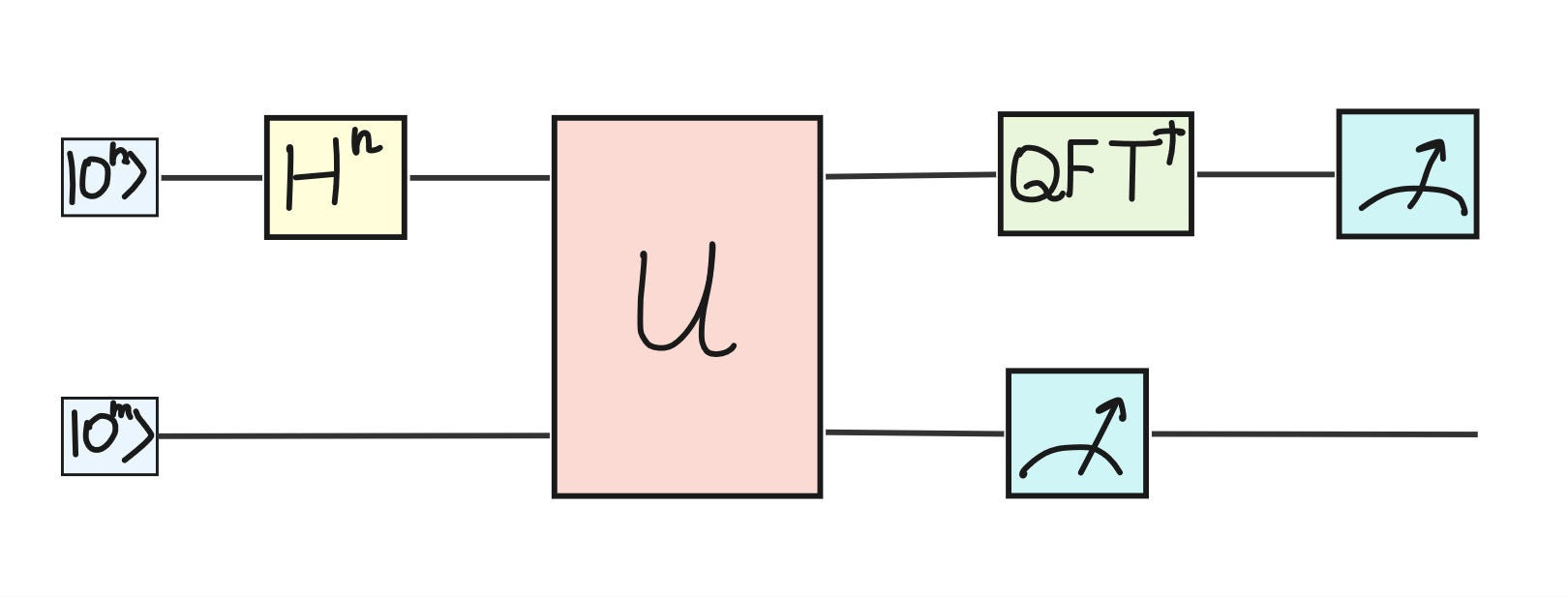
Step 1. As it is conventional in quantum computing, we start the algorithm with initial quantum state with all qubits in the state |0>. We will split all qubits in the following way: the first several qubits will encode the counting register (denoted |i>) and the rest will encode the result of the period finding (denoted |a^i mod K>).
Step 2. We apply Hadamard gates on the counting registers only to bring them into an equal superposition.

Step 3. On this stage of the algorithm, we act with a unitary U such that on the second quantum register we will obtain the states |a^i mod K> — the result of the modulo division.

Note: we assume here that we know the unitary operator U in advance. When designing the factoring algorithm, however, this unitary U can be represented by a sequence of control-rotation quantum gates.
Additionally, the number 8 in the denominator occurs because I chose 3 qubits in the counting register so 2³ = 8. For an educational example, 3 qubits are fair play. Nevertheless, if running Shor’s factoring algorithm on quantum hardware, we want to consider more qubits to increase the success probability of the algorithm.
After applying the unitary U, we will get the counters in the first register: 0, 1, 2, … 7. The second register contains the result of modulus division.

At this step, some interesting things start happening: after careful observation, you can notice that the values in the second quantum register repeat: 1, 5, 25, 8, 1, 5, 25, 8. If we consider a larger N in the sum, this pattern remains. In fact, you can verify this observation by writing a simple Python for loop of the expression |5^i mod 39> (feel free to change N as you like):
N = 40
for i in range(0, N):
  print(5 ** i % 39, end=" ")

>>> 1 5 25 8 1 5 25 8 1 5 25 8 1 5 25 8 1 5 25 8 1 5 25 8 1 5 25 8 1 5 25 8 1 5 25 8 1 5 25 8
Step 4. At this step, we measure the second register only. Observe, that there is an equal probability of obtaining either |1> or |5> or |25>, or |8>. Let’s say we find that the second register is in the state |1>. Then, the entanglement between the first and second quantum register disappears and we observe only corresponding to the |1> numbers in the counting register. That is, we observe the superposition of |0> and |4> states.
Mathematically, we get (don’t forget to re-normalize the state):

Step 5. At this step, we apply the inverse of the QFT (Quantum Fourier Transform) on the first register. The QFT allows to amplify information needed and cancel out all unimportant bits. We will use the following formula:

For example, if the inverse of the QFT acts on the |0> state then we get

Similarly, if the inverse of the QFT acts on the |4> state, we get

Now, since we still have |0> and |4> in equal superposition, we add the results of applying the inverse of Quantum Fourier Transformation to these states, keeping in mind the normalization factor of 1/√2:

Upon careful examination of the expression inside the parenthesis, we can factor out 1/√8, the ket |m>, and alter the summation method without affecting the result:

Before we iterate over m = 0, 1, …, 7 in the sum, we can separately examine the expression

where the Euler’s formula was applied. Since m is an integer from 0 to 7, the sin(𝞹m) = 0 for all m values. The cos(𝞹m), on the other hand, can be either 1 for even values of m or -1 for odd values of m. For each even value of m, the sum (1+exp(-𝞹im) is 2; for each odd value of m, the sum (1+exp(-𝞹im) is 0. So we can observe constructive interference for even m’s and destructive interference for odd m’s:

As a result, upon obtaining measurement distribution, we get an equal superposition of 0, 2, 4, and 6. Note: 0 is a trivial solution that we are not interested in. So we can safely omit it.
Step 6. Our next several calculations are classical postprocessing of our results. We calculate the Greatest Common Divisor (GCD) of the measured numbers:

Now, we return back to the formulas from Step 0.

GCD(39, 24) = 3. Here we go, c=3 is the first prime factor of 39! Now, we repeat for the other factor:

GCD(39, 26) = 13=d which is the second prime factor of 39!
Congrats! You have successfully factored out a number using Shor’s factoring algorithm.
Reference
M.A. Nielsen, I.L. Chuang. Quantum Computing and Quantum Information. Cambridge University Press, 2016.
Skosana, U., Tame, M. Demonstration of Shor’s factoring algorithm for N 21 on IBM quantum processors. Sci Rep 11, 16599 (2021). https://doi.org/10.1038/s41598-021-95973-w
All opinions and views are my own and do not reflect opinions of my current, past, or future employers.
If you like my stories and want to learn more about the Quantum field, please clap (lots!!), leave a comment, and buy me a cup of tea.